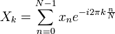
When I was trying to understand how the Fourier Transform worked, it took me days of reading before it finally clicked. Now that I understand it, the formula seems incredibly simple. The goal of this article is to hopefully present a simple description of how the formula works.
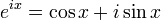
At first glance, the formula appears very complicated, mostly due to the exponential raised to a complex power. Once it is understood what the exponential is doing, the formula becomes much more logical and easily followed. The first step is to modify the expression using Euler's formula:
Replacing into the Fourier Transform yields:
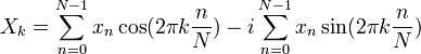
The formula is now broken into two summations, one to determine how well a cosine wave matches the signal and another to determine how well a sine wave matches the signal. Since the calculations are the same for both summations, let us focus only on the cosine term in order to simplify the example:
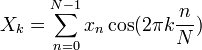
Written in English, the formula states: to find the strength of the
signal at  Hz (
Hz ( ), multiply the value of
the signal (
), multiply the value of
the signal ( ) times the value of a cosine wave at
Hz (
) times the value of a cosine wave at
Hz ( ) at the same point in time
(
) at the same point in time
( ). Sum all of the multiplied values up.
Basically, the formula overlays an ideal signal () on top of the real signal and computes how closely the ideal
signal compares.
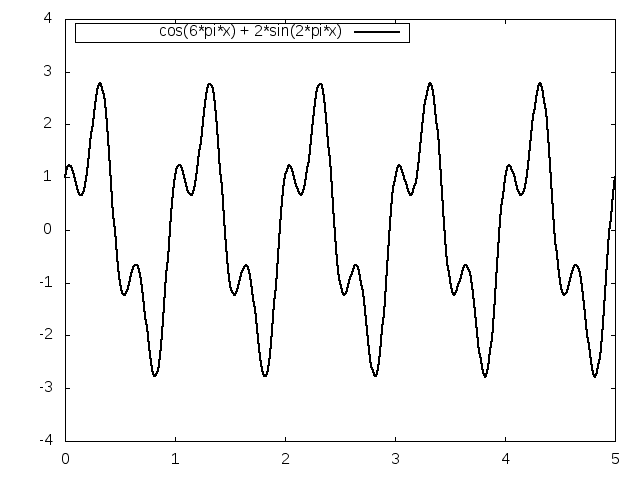
Let us look at an example: Suppose we have a signal that is composed of a combination of a cosine wave at 3 Hz with amplitude 1 and a sine wave at 1 Hz with amplitude 2:

Let us now see how well the signal matches against a 1 Hz cosine wave:
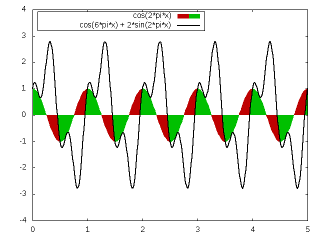
The areas in green show where the multiplication of the signal and the cosine wave results in a positive value. The areas in red show negative values. When the areas are added together, they result in a value close to zero. This means that a 1 Hz cosine wave does not match this signal well.
Next, let us look to see how well the signal matches against a 3 Hz cosine wave:
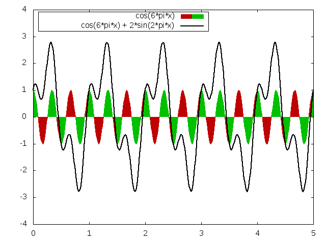
In this case, there are many more areas with green than there are red. This means that a 3 Hz cosine wave does match this signal well.
The full transform can be computed by following the formula. The table below was produced using a sample size of 10 (remember the Nyquist Theorem which states that the sampling rate must be twice the maximum frequency; a sample size of 10 means that we can only reproduce a maximum frequency of 5 Hz). The code to calculate these results in listed in Appendix A.
| Hz | Cosine | Sine | Magnitude |
|---|---|---|---|
| 0 | 0 | 0 | 0 |
| 1 | 0 | -2 | 2 |
| 2 | 0 | 0 | 0 |
| 3 | 1 | 0 | 1 |
| 4 | 0 | 0 | 0 |
| 5 | 0 | 0 | 0 |
The following C program computes the Fourier Transform as shown in the Example section.
#include <stdio.h>
#include <stdlib.h>
#include <math.h>
#include <complex.h>

/* Calculates the Discrete Fourier Transform in O(n^2) time. */
void dft(double complex *in, double complex *out, size_t len)
{
    int k, n, N;
    double complex c, c2;
    double complex sum;
    double arg;

    N = len;

    for (k = 0; k < N; k++) {
        sum = 0;
        for (n = 0; n < N; n++) {
            c = cexp(-I * 2 * M_PI * k * n / N);
            sum += in[n] * c;
        }
        out[k] = sum;
    }
}

int main()
{
    const int samples = 10;
    double complex values[samples];
    double complex result[samples];
    int i;

    /* Create the signal cos(6*pi) + 2*sin(2*pi). */
    for (i = 0; i < samples; i++)
        values[i] = cos(6 * M_PI * i / samples)
            + 2 * sin(2 * M_PI * i / samples);

    /* Compute the Fourier Transform. */
    dft(values, result, samples);

    /* Display the results. */
    printf("Hz    cos    sin    magnitude\n");
    printf("-----------------------------\n");
    for (i = 0; i < samples / 2 + 1; i++) {
        /*
         * The Fourier Transform produces a scaled result.
         * Divide by the number of samples to see the correct
         * amplitudes.
         */
        result[i] /= samples / 2;

        printf("%2d  %5.1f  %5.1f  %11.1f\n", i, creal(result[i]),
               cimag(result[i]), cabs(result[i]));
    }

    return 0;
}

/*
 * The output of the program:
 *
 * Hz    cos    sin    magnitude
 * -----------------------------
 *  0    0.0    0.0          0.0
 *  1    0.0   -2.0          2.0
 *  2   -0.0    0.0          0.0
 *  3    1.0    0.0          1.0
 *  4    0.0   -0.0          0.0
 *  5    0.0   -0.0          0.0
 */